TL;DR🔗
- You can use the library collection Tidyverse, to draw and customize Gantt charts from batsim simulations.
- For Batsim > 3.0 you may need to change
allocated_resourcestoallocated_processors. - You can use the function below to skip everything and start plotting
library(tidyverse)

draw_gantt <- function(workload_path) {

  workload <- read_csv(workload_path)
  # Data processing to have a ggplot friendly formatting
  workload_sep <- workload %>%
    # We split the jobs into one row per allocation bloque
    separate_rows(allocated_processors, sep=" ") %>%
    # We create two columns, one for the block (min resource and max)
    separate(allocated_processors, into = c("psetmin", "psetmax"), fill="right") %>%
    mutate(psetmax = as.integer(psetmax), psetmin = as.integer(psetmin)) %>%
    mutate(psetmax = ifelse(is.na(psetmax), psetmin, psetmax))

  # Start ploting
  workload_sep  %>%
    ggplot(aes( xmin=starting_time,
                ymin=psetmin,
                ymax=psetmax + 0.9,
                xmax=finish_time,
                fill=workload_name)) +
    # We draw the rectangle
    geom_rect(alpha=0.6,color="black", size=0.1) +
    # We add the label in the middle of the block
    geom_text(aes(x=starting_time +(finish_time-starting_time)/2, # size=stretch,
                y=psetmin+((psetmax-psetmin)/2)+0.5,
                label=paste(job_id, "")), alpha=1,check_overlap = TRUE) +
    # We add the segment at the bottom of the gantt
    geom_segment(
      aes(x=submission_time,
          y=psetmin+0.1,
          xend=starting_time,
          yend=psetmax
          ),
      alpha=1,
      size=0.1) +
    # On a white background
    theme_bw() +
    ylab("resources") + xlab("time (in seconds)") + theme(legend.position = "none") +
    scale_color_viridis(discrete=F) + scale_fill_viridis(discrete=T)
}
The files🔗
Batsim🔗
Batsim is a simulator essentially developed into my team at the laboratory of Grenoble.
To describe it simply, batsim is a simulator of batch scheduler designed for distributed platforms, such as an High Performance Computing cluster. Its strength lies in the ease to design scheduling algorithm in any languages, thanks to a network API.
However, this post does not focus on how to use batsim but on how we can leverage the great ggplot2 API to draw a Gantt chart from output simulations. I will therefore assume that you already know batsim and how to use it. For more informations, you can always refer to the documentation, or send me an email :) .
Visualisations🔗
R and ggplot2🔗
Ggplot2, is a R library designed to plot data, it comes within a collection of R library called Tidyverse. Tidyverse is very handy when it comes to data manipulations. One can cite:
- readr that loads data and detect anomalies, formatting etc.
- dplyr for data manipulations.
- ggplot2 for visualizations.
I wont go in any details on the design and architecture of these libraries, however if you are interested to go further into it, the related book (R for datascience) can be a good point to start.
library(tidyverse) # Tidyverse library collection
library(viridis) # Nice color palette
Gantt charts🔗
When doing experiments on complicated problems such as scheduling, we need to understand what is happening. You can use statistics, but in some cases it may give you intuitions on what is happening. However your answer may lie in the details. Thankfully, to study scheduling we can use Gantt charts which is a 2D representation of tasks, resources and time.
The example below shows an example of a Gantt chart made with gglot2. Every chart created in this plot are reproducible, and the file that contains the job is available here.
Evalys🔗
Evalys is a python library to deal with batsim output, and workloads of HPC jobs. Evalys, has a real application structures, and proposes a lot of other visualisations, such as the load of the system, the size of the queue. If you are more a python person, I suggest to directly use evalys.
In my case, many of my scripts and visualisations of my workflow are in R. So to limit the number of ecosystems I need to use, I choose to plot my gantt in R.
From batsim output to gantt🔗
The first thing to do is to set up your R environment, for that you can install R and the libraries I introduced earlier. The installation details are detailed here: https://www.tidyverse.org/packages/.
Once the installation is done, we can start to work with the data. The next thing you need is an output from batsim, in this blog I use an output from one of my simulations. You can download it here if you want to play with it.
We can load the jobs with the following block code and explore the data.
workload <- read_csv("jobs.csv")

# Print the colnames
colnames(workload)
##  [1] "job_id"                         "hacky_job_id"
##  [3] "workload_name"                  "submission_time"
##  [5] "requested_number_of_processors" "requested_time"
##  [7] "success"                        "starting_time"
##  [9] "execution_time"                 "finish_time"
## [11] "waiting_time"                   "turnaround_time"
## [13] "stretch"                        "consumed_energy"
## [15] "allocated_processors"
# Print a few lines
head(workload)
## # A tibble: 6 x 15
##   job_id hacky_job_id workload_name submission_time requested_number_of_p…
##    <int>        <int> <chr>                   <dbl>                  <int>
## 1      0            0 0e8208                      0                     10
## 2      1           10 0e8208                    681                      4
## 3      2           20 0e8208                   3095                     16
## 4      3           30 0e8208                   3260                      1
## 5      4           40 0e8208                   3467                     16
## 6      5           50 0e8208                   8360                      4
## # ... with 10 more variables: requested_time <dbl>, success <int>,
## #   starting_time <dbl>, execution_time <dbl>, finish_time <dbl>,
## #   waiting_time <dbl>, turnaround_time <dbl>, stretch <dbl>,
## #   consumed_energy <dbl>, allocated_processors <chr>
In this CSV, each line is the record of a job. Each job has a submission
time, a starting time, an execution time etc. One important column is
the allocated_processors which correspond to the resources that have
been allocated to the job. The format is the following: “0 3-5 10-15”,
which means that the job was executed on the processors 0 3 4 5 10 11 12
13 14 15. It is an important information as it the y axis of a Gantt.
Now that we loaded the data, we want two print each jobs on a grid to create the gantt chart.
However, the formatting of the allocated_processor does not directly give informations processable with ggplot2. Indeed, in order to be able to plot several squares by jobs, ggplot2 needs that we create as many rows as squares. Thus one row per job is not sufficient.
For example the job 29 holds the resources from 0 to 11 and from 28 to 43.
# I extract two jobs as an illustration
# but the following will use these two jobs as an example.
three_jobs <- workload %>% filter(job_id == 29 | job_id == 27 | job_id == 33)
three_jobs %>% select(job_id, allocated_processors)
## # A tibble: 3 x 2
##   job_id allocated_processors
##    <int> <chr>
## 1     27 12-27
## 2     29 0-11 28-43
## 3     33 0-11 28-43
Basically, we need to draw a square by non-contiguous set of resources of a job. The solution is to split each jobs in rows (one row per square).
Thankfully it is easy with tidyverse.
I use the two following functions:
separate_rowsthat split a rows in one or several rows according to a separator (a simple space in our case). We see that the jobs 29 and 33 now appear two times
chunk <- three_jobs %>%
   separate_rows(allocated_processors, sep=" ")

# print the result
chunk %>% select(job_id, allocated_processors)
## # A tibble: 5 x 2
##   job_id allocated_processors
##    <int> <chr>
## 1     27 12-27
## 2     29 0-11
## 3     29 28-43
## 4     33 0-11
## 5     33 28-43
separatethat split a column in one or several columns. We use this last transformation to create a column psetmax and psetmin that contains the resources min (the bottom of our square) and max (the top).
chunk <- chunk %>%
   separate(allocated_processors, sep="-", into = c("psetmin", "psetmax"), fill="right") %>%
   # A last transformation in case of single resource, we set the max as the min.
   mutate(psetmax = as.integer(psetmax), psetmin = as.integer(psetmin)) %>%
   mutate(psetmax = ifelse(is.na(psetmax), psetmin, psetmax))

# Display the result
chunk
## # A tibble: 5 x 16
##   job_id hacky_job_id workload_name submission_time requested_number_of_p…
##    <int>        <int> <chr>                   <dbl>                  <int>
## 1     27          270 0e8208                 107474                     16
## 2     29          290 0e8208                 111742                     28
## 3     29          290 0e8208                 111742                     28
## 4     33          330 0e8208                 113219                     32
## 5     33          330 0e8208                 113219                     32
## # ... with 11 more variables: requested_time <dbl>, success <int>,
## #   starting_time <dbl>, execution_time <dbl>, finish_time <dbl>,
## #   waiting_time <dbl>, turnaround_time <dbl>, stretch <dbl>,
## #   consumed_energy <dbl>, psetmin <int>, psetmax <int>
Once we did that, we can start to plot our Gantt using the
geom_rect
function.
chunk  %>%
  # We pipe chunk that contains our three jobs into ggplot
  ggplot(aes( xmin=starting_time,
                  ymin=psetmin,
                  ymax=psetmax + 0.9,
                  xmax=finish_time,
                  fill=workload_name)) +
  # We add the rectangles
  geom_rect(color="black", size=0.5, alpha=0.5) +
  # We also add a label
  geom_text(aes(x=starting_time +(finish_time-starting_time)/2,
                y=psetmin+((psetmax-psetmin)/2)+0.5,
                label=paste(job_id, "")), alpha=1,check_overlap = TRUE) +
  scale_color_viridis(discrete=F) + scale_fill_viridis(discrete=T) +
  # We rename our labels
  ylab("resources") + xlab("time (in seconds)") + theme_bw() + theme(legend.position = "none")
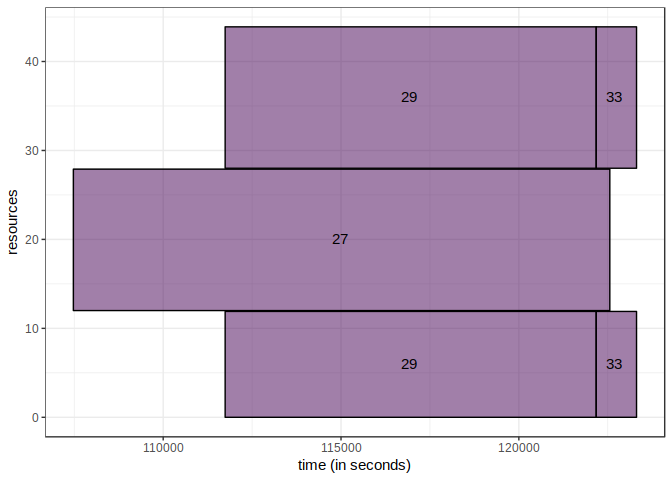
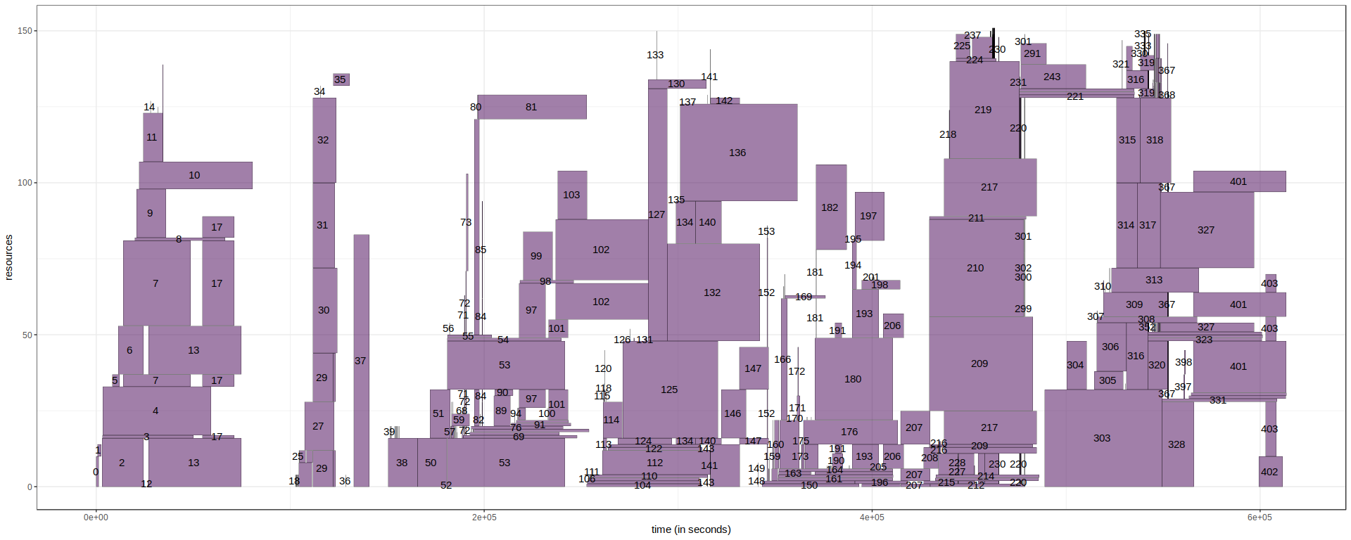
And now we can plot the whole set of job.
workload_sep <- workload %>%
  separate_rows(allocated_processors, sep=" ") %>%
  separate(allocated_processors, into = c("psetmin", "psetmax"), fill="right") %>%
  mutate(psetmax = as.integer(psetmax), psetmin = as.integer(psetmin)) %>%
  mutate(psetmax = ifelse(is.na(psetmax), psetmin, psetmax))

workload_sep %>%
  ggplot(aes(xmin=starting_time,
                  ymin=psetmin,
                  ymax=psetmax + 0.9,
                  xmax=finish_time,
                  fill=workload_name)) +
  scale_color_viridis(discrete=F) + scale_fill_viridis(discrete=T) +
  geom_rect(color="black", size=0.1, alpha=0.5) +
  geom_text(aes(x=starting_time +(finish_time-starting_time)/2,
                y=psetmin+((psetmax-psetmin)/2)+0.5,
                label=paste(job_id, "")),
            alpha=1, check_overlap = TRUE) +
  # add some theming options
  theme_bw() + theme(legend.position =  "none") +
  ylab("resources") + xlab("time (in seconds)")
Adapt to your case🔗
At this point, we know how to plot a set of job as a gantt chart, great! From this point, we have all the cards to create a plot adapted to your need. And this in where I think that we best take advantage of ggplot2.
Disclaimer:
This section is not meant to be exhaustive, but rather a set of ideas and transformation I performed on the gantt thanks to ggplot to suit to my case. Many idea are extracted from the library evalys, which I introduced at the beginning of this post.
Shows workload activity🔗
This visualisation is directly taken from evalys :) We add, under the gantt, a line for each jobs of the workload.
Lets try this on a few jobs.
Each job has a segment, and each segment has two point, starting from the bottom, it is the submit time of a job to the top of the segment its running time. Thus, the inclination of a segment gives an indication of the waiting time of a job. If the segment is vertical, it means that the job has been directly launched.
With the gantt below, we see that the job 33 waited before being launched.
chunk  %>%
  ggplot(aes( xmin=starting_time,
              ymin=psetmin,
              ymax=psetmax + 0.9,
              xmax=finish_time,
              fill=workload_name)) +
  scale_color_viridis(discrete=F) + scale_fill_viridis(discrete=T) +
  # The main rectangle
  geom_rect(alpha=0.4, color="black", size=0.7) +
  # The label
  geom_text(aes(x=starting_time +(finish_time-starting_time)/2,
                y=psetmin+((psetmax-psetmin)/2)+0.5,
                label=paste(job_id, "")), alpha=1,check_overlap = TRUE) +
  # The segment under the gantt
  geom_segment(aes(x=submission_time,
                   y=-17,
                   xend=starting_time,
                   yend=-3), size=0.1) +
  geom_point(aes(y=-17, x=submission_time), size=0.1) +
  geom_point(aes(y=-3, x=starting_time)) +
  theme_bw() + theme(legend.position = "none") +
  ylab("resources") + xlab("time (in seconds)")
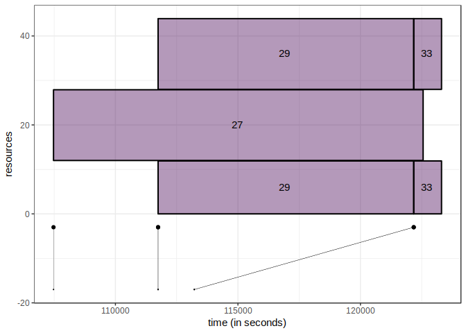
If in this case it remains simple to associate the last segment with the job 33, it becomes more difficult with more jobs. However, it gives a good idea of the intensity of the workload.
workload_sep  %>%
  ggplot(aes( xmin=starting_time,
              ymin=psetmin,
              ymax=psetmax + 0.9,
              xmax=finish_time,
              fill=workload_name)) +
        scale_color_viridis(discrete=F) + scale_fill_viridis(discrete=T) +
  # The main rectangle
  geom_rect(alpha=0.4, color="black", size=0.7) +
  # The label
  geom_text(aes(x=starting_time +(finish_time-starting_time)/2,
              y=psetmin+((psetmax-psetmin)/2)+0.5,
              label=paste(job_id, "")), alpha=1,check_overlap = TRUE) +
  # The segment under the gantt
  geom_segment(aes(x=submission_time,
        y=-40,
        xend=starting_time,
        yend=-3), size=0.1) +
  geom_point(aes(y=-40, x=submission_time), size=0.1) +
  geom_point(aes(y=-3, x=starting_time)) +
  theme_bw() + theme(legend.position = "none") +
  ylab("resources") + xlab("time (in seconds)")

We could go even further, and adapt the size and the intensity of the color of jobs that has a high waiting_time.
workload_sep  %>%
  ggplot(aes( xmin=starting_time,
              ymin=psetmin,
              ymax=psetmax + 0.9,
              xmax=finish_time,
              # here it will set the alpha globaly
              alpha=waiting_time,
              fill=workload_name)) +
        scale_color_viridis(discrete=F) + scale_fill_viridis(discrete=T) +
  # This draw the rectangles
  geom_rect(color="black", size=0.1) +
  # And we add the labels of the job id
  geom_text(aes(x=starting_time +(finish_time-starting_time)/2, # size=stretch,
              y=psetmin+((psetmax-psetmin)/2)+0.5,
              label=paste(job_id, "")), alpha=1,check_overlap = TRUE) +

  geom_point(aes(y=psetmin+0.5, x=submission_time), size=0.0001) +
  geom_segment(aes(x=submission_time,
        y=-50,
        xend=starting_time,
        yend=-3), size=0.1) +
  geom_point(aes(y=-50, x=submission_time), size=0.1) +
  geom_point(aes(y=-3, x=starting_time), size=0.1) +
  theme_bw() +
  ylab("resources") + xlab("time (in seconds)")
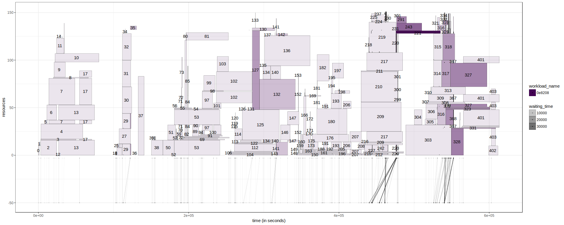
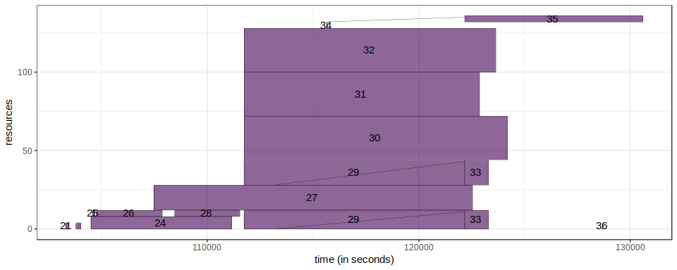
One last thing we can do, in replacement of the segment below the gantt, is to add the segment directly to the gantt chart, such as:
With this visualisation, it becomes easier to identify jobs and see when see have been submitted (But we loose the vision on the overall workload).
workload_sep  %>%
  ggplot(aes( xmin=starting_time,
              ymin=psetmin,
              ymax=psetmmax + 0.9,
              xmax=finish_time,
              fill=workload_name)) +
        scale_color_viridis(discrete=F) + scale_fill_viridis(discrete=T) +
  geom_rect(aes(alpha=waiting_time),color="black", size=0.1) +
  geom_text(aes(x=starting_time +(finish_time-starting_time)/2, # size=stretch,
              y=psetmin+((psetmax-psetmin)/2)+0.5,
              label=paste(job_id, "")), alpha=1,check_overlap = TRUE) +
  geom_segment(
    aes(x=submission_time,
        y=psetmin+0.1,
        xend=starting_time,
        yend=psetmax
        ),
    alpha=1,
    size=0.1) +
  theme_bw() +
  ylab("resources") + xlab("time (in seconds)")

Zooming🔗
When a plot is too loaded, we can consider zooming on a particular slice of the gantt.
# From sec
from = 500000
# to the terminason of the last job
to = max(workload$finish_time)

workload_sep  %>% # filter(submission_time >  time | execution_time > time | finish_time > time) %>%
  ggplot(aes( xmin=starting_time,
              ymin=psetmin,
              ymax=psetmax + 0.9,
              xmax=finish_time,
              fill=workload_name)) + coord_cartesian(xlim=c(from, to)) +
        scale_color_viridis(discrete=F) + scale_fill_viridis(discrete=T) +
  geom_rect(aes(alpha=waiting_time),color="black", size=0.1) +
  geom_text(aes(x=starting_time +(finish_time-starting_time)/2, # size=stretch,
              y=psetmin+((psetmax-psetmin)/2)+0.5,
              label=paste(job_id, "")), alpha=1,check_overlap = TRUE) +
  geom_segment(
    aes(x=submission_time,
        y=psetmin+0.1,
        xend=starting_time,
        yend=psetmax
        ),
    alpha=1,
    size=0.1) +
    geom_point(aes(y=psetmin+0.5, x=submission_time), size=0.0001) +
  geom_segment(aes(x=submission_time,
        y=-50,
        xend=starting_time,
        yend=-3), size=0.1) +
  geom_point(aes(y=-50, x=submission_time), size=0.1) +
  geom_point(aes(y=-3, x=starting_time), size=0.1) +
  theme_bw() +
  ylab("resources") + xlab("time (in seconds)")

Conclusion🔗
In this post, I showed how we can use ggplot2 to draw gantt from a batsim output. It becomes clear that it is a powerful tool to allow us what happens is our simulations.
As I said in the previous section, it is not exhaustive list of we can do with ggplot2 to draw gantt, so I am open to new ideas :)
You can download this file as a notebook to replay it.